SyntenyPlotteR - a tool for genome synteny visualisation
Source:vignettes/syntenyPlotteR.Rmd
syntenyPlotteR.RmdIntroduction
Determining syntenic relationships between genomes is a important step in understanding genome evolution. To do this, researchers align species genomes to one another to detect sequence markers and conserved sequences to identify syntenic regions. There is a plethora of tools which can be used to identify this synteny such as DESCHRAMBLER. However, they often return tables showing the orientation and, start and stop positions of the syntenic regions which can often be hard to interpret at face value.
Here, we provide a tool which visualises this data, improving the
interpretation of the alignment data, particularly for the
identification, characterization, and visualization of chromosome
rearrangements. SyntenyPlotteR relies on the use of ggplot2 to create
the graphics, producing three potential visualizations: a linear
relationship between syntenic regions of the genome using
draw.linear(), an evolution highway style grid showing
synteny between single chromosomes aligned between a single reference
species and one or more target species using draw.eh(), and
an ideogram with painted chromosomes to show syntenic relationships
between two genomes using draw.ideogram(). There is also a
function which can reformat data structured in the
DESCHRAMBLER/inferCARs format to a structure suitable for the required
input to the aforementioned functions using
reformat.syntenyData().
SyntenyPlotteR is solely designed to plot synteny data already gathered by the user. This tool does not generate syntenic relationships or curate data. As such, the user is required to construct syntenic blocks, therefore, allowing the user to choose the most appropriate tool for their needs. SyntenyPlotteR is easily implemented by the user with single line functions taking directly the tab delimited files containing the alignment data and chromosome lengths, thus meaning even inexperienced users find the process fast to learn and simple to use.
This package has been developed by Sarah Quigley (slq4@kent.ac.uk), Joana Damas (joanadamas@gmail.com), Denis Larkin (dlarkin@rvc.ac.uk) and Marta Farré (m.farre-belmonte@kent.ac.uk)
Input files
Alignment output file format for reformat.syntenyData()
function
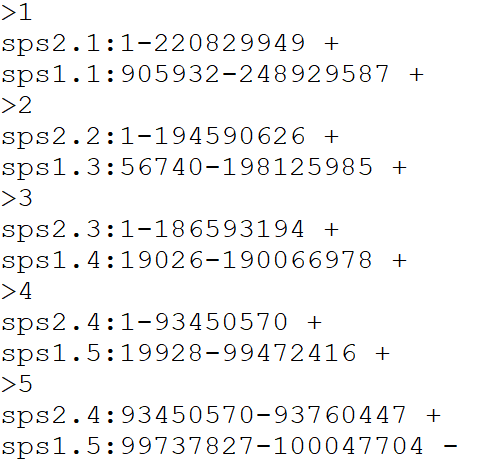
If chromosome alignment was performed using DESCHRAMBLER please input the .map file If chromosome alignment was performed using inferCARs please input the inferCARs output file
Alignment file input format for draw.eh(),
draw.ideogram(), and draw.linear()
functions
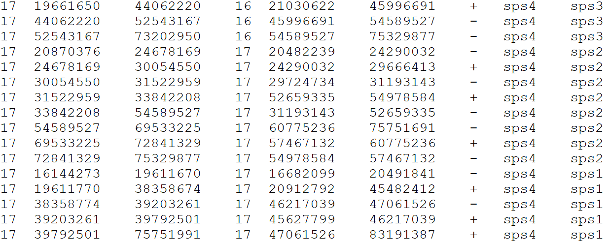
Please provide a file for the alignment synteny blocks following this format, separated by tabs
DO NOT include a header line
- Reference chromosome ID
- Reference start position
- Reference end position
- Target chromosome
- Target start position
- Target end position
- Orientation
- Reference species ID
- Target species ID
Example file format

Chromosome Length file for draw.ideogram() and
draw.linear() functions
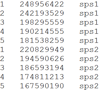
Please provide a file containing all aligned species in order from first target species in the alignment files followed by the first reference species in the alignment files – top of file – to the last target species and reference species in the alignment files – end of file, following this format, separated by tabs.
Note: the order you input the species in the length file
determines the order of which the species will be placed in the
draw.linear() function; for example the first species in
the length file (top of file) will be the first linear genome drawn thus
at the bottom of the Y axis. In the case of aligning two target species
to a single reference species, it is suggested you place the reference
in the middle of the length file - i.e. target 1 (top of file),
reference (middle of file), target 2 (bottom of file).
DO NOT include a header line
- Chromosome ID
- Chromosome length
- Species ID
Reformatting alignment data
The syntenyPlotteR package includes a function to reformat alignment synteny data such as from DESCHRAMBLER or inferCARs - this does not curate files only reformats it
The function outputs a text file containing the reformatted alignment
data. As default the function saves the file to a temporary directory,
this can be overridden using the directory parameter
i.e. directory = "path/to/directory".
Usage
library(syntenyPlotteR)

reformat.syntenyData("file_data", "output.filename", reference.species = "reference.sps", target.species = "target.sps")- file_data - alignment output file from DESCHRAMBLER/infeCARs
- output.filename - output file name for reformatted data in a character string
There are optional parameters for some customization of this function:
- reference.species - reference species ID as character string for final output table
- target.species - target species ID as character string for final output table
- directory - directory where to save text file
i.e.
directory = "path/to/directory"
Example code using data files in inst/extdata/
reformat.syntenyData("example_map_1.map", "reformatted.data")Evolution Highway style
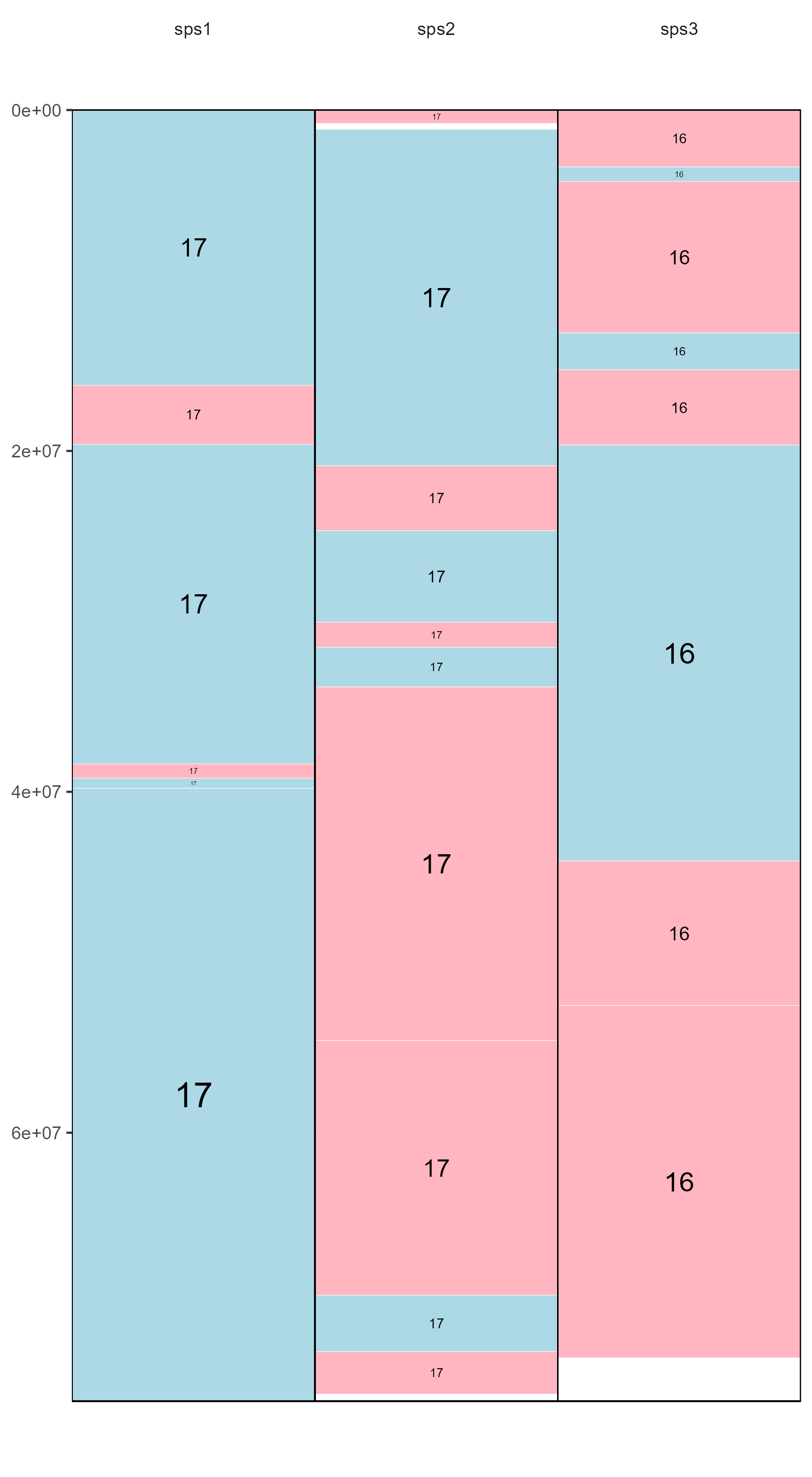
The function outputs an image file containing the evolution highway
style alignment. As default the function saves the file to a temporary
directory, this can be overridden using the directory
parameter i.e. directory = "path/to/directory".
Usage
library(syntenyPlotteR)

draw.eh("output", chrRange, "data_file", fileformat = "png", colour = "lightblue", inverted.colour = "lightpink", w = 5.5, h = 10, ps = 10)- output - String assigned to name of output file name
- chrRange - The range of chromosomes of the reference species this is entered as either a single number i.e. 1 or a range of numbers i.e. 1:22. Note: if you are inputting sex chromosomes or chromosomes with characters in the name input a concatenated string i.e. c(1,2,3,“X”)
- data_file - File containing the syntenic blocks of alignments of one or more target species aligned to a single reference
There are optional parameters for some customization of this function:
- fileformat - format for saving the image i.e. png or pdf, parameter
use:
fileformat = "pdf"(the default value is “png”) - colour - colour of the syntenic blocks (not inverted blocks),
parameter use:
colour = "red"(the default value is “lightblue”, see Rcolour pallette for colour options) - inverted.colour - colour of the inverted syntenic blocks, parameter
use:
inverted.colour = "blue"(the default value is “lightpink”, see Rcolour pallette for colour options) - w - The width of the image created can be changed by using:
w = 5.5(default) - h - The height of the image created can be changed by using:
h = 10(default) - ps - The point size of the image created can be changed by using:
ps = 10(default) - directory - directory where to save image file
i.e.
directory = "path/to/directory"(default is save to temporary directory)
Example output:
Chromosome painting style
The function outputs an image file containing the chromosome painting
style alignment. As default the function saves the file to a temporary
directory, this can be overridden using the directory
parameter i.e. directory = "path/to/directory".
Usage
library(syntenyPlotteR)

draw.ideogram("file_data", "sizefile", "output", fileformat = "png", colours = colours.default, w=8.5, h=10, ps=5)- file_data - file containing the syntenic blocks
- sizefile - tab separated file of all chromosome, scaffold, or contig lengths and the species identifier, in order from first target species in the alignment files followed by the first reference species in the alignment files – top of file – to the last target species and reference species in the alignment files – end of file.
- output - string assigned to the output file name
There are optional parameters for some customization of this function:
- fileformat - format for saving the image i.e. png or pdf, parameter
use:
fileformat = "pdf"(the default value is “png”) - colours - colours to assign to the ideograms in a concatenated
string of chromosome IDs with assigned colour values which can be found
with R colour Pallette, paramter use:
colours = c("1" = "red", "2" = "blue", "3" = "green","4" = "orange", "5" = "purple","X" = "grey")if no colours are assigned default values will be used but colours MUST be assigned to all chromosomes - w - The width of the image created can be changed by using:
w = 5.5(default) - h - The height of the image created can be changed by using:
h = 10(default) - ps - The point size of the image created can be changed by using:
ps = 10(default) - directory - directory where to save image file
i.e.
directory = "path/to/directory"(default is save to temporary directory)
Target is the species which chromosomes will be painted. Reference will be used for painting and diagonals. Chromosomes will be in the same order as in the target sizes file.
Note: If you have any alignments with chromosomes not defined in the length file the function will not run.
Example code using data files in inst/extdata/
draw.ideogram("example_alignment_1.txt", "example_lengths.txt", "example.ideogram")Example output:

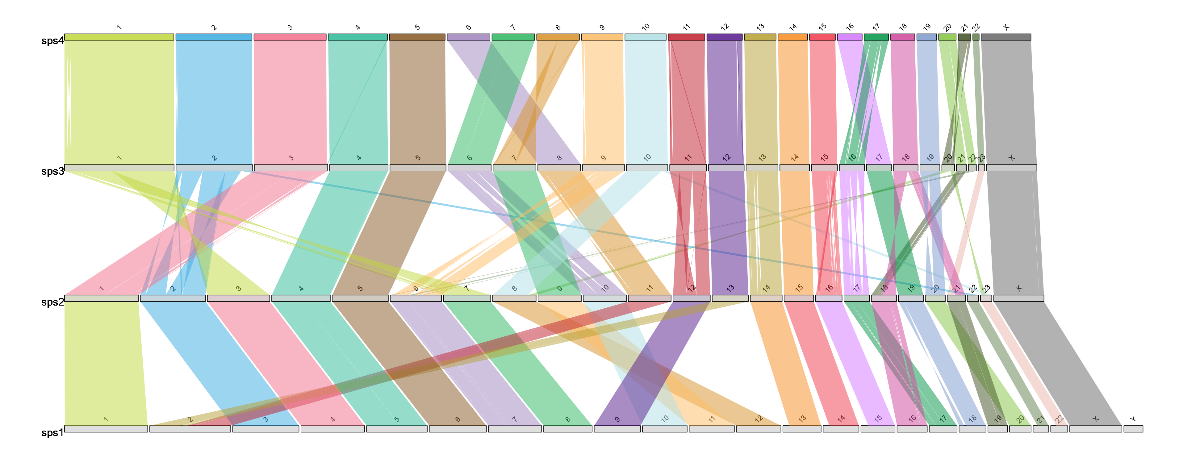
Linear style
The function outputs an image file containing the linear style
alignment. As default the function saves the file to a temporary
directory, this can be overridden using the directory
parameter i.e. directory = "path/to/directory".
Usage
library(syntenyPlotteR)

draw.linear(output, sizefile, ..., fileformat = "png", colours = colours.default, w=13, h=5, opacity = .5)- output - string assigned to the output file name
- sizefile - tab separated file of all chromosome, scaffold, or contig lengths and the species identifier, in order from first target species in the alignment files followed by the first reference species in the alignment files – top of file – to the last target species and reference species in the alignment files – end of file.
- … - files containing the syntenic blocks (one file per alignment, in order from first target/reference (most recent species pairwise alignment in ancestral reconstruction data) alignment file to last target/reference (ancestor pairwise alignment in ancestral reconstruction data) alignment file)
Please ensure any species identifiers used between length and alignment files are matching (same identifiers and letter case)
There are optional parameters for some customization of this function:
- fileformat - format for saving the image i.e. png or pdf, parameter
use:
fileformat = "pdf"(the default value is “png”) - colours - colours to assign to the bands between ideograms in a
concatenated string of chromosome IDs with assigned colour values which
can be found with R colour Pallette, paramter use:
colours = c("1" = "red", "2" = "blue", "3" = "green","4" = "orange", "5" = "purple","X" = "grey")if no colours are assigned default values will be used but colours MUST be assigned to all chromosomes - w - The width of the image created can be changed by using:
w = 5.5(default) - h - The height of the image created can be changed by using:
h = 10(default) - opacity - the opacity of the ribbons can be changes using inputting:
opacity = .5(default) - directory - directory where to save image file
i.e.
directory = "path/to/directory"(default is save to temporary directory)
Note: If you have any alignments with chromosomes not defined in the length file the function will not run.
Example code using data files in inst/extdata/
draw.linear("example_linear", "example_lengths.txt", "example_alignment_1.txt", "example_alignment_2.txt", "example_alignment_3.txt")Example output:
